7. A simple example with HMM

python file

In this example, we will:

Create a HMM H from scratch,
Use it to generate a training set,
Use the Baum-Welch algorithm to learn, from the training set, H,
Compare H with the output model.

Creating a HMM

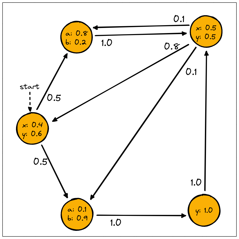
We can create the model depicted above like this:

>>> import jajapy as ja
>>> transitions = [(0,1,0.5),(0,2,0.5),(1,3,1.0),(2,4,1.0),
>>>                        (3,0,0.8),(3,1,0.1),(3,2,0.1),(4,3,1.0)]
>>> emission = [(0,"x",0.4),(0,"y",0.6),(1,"a",0.8),(1,"b",0.2),
>>>                     (2,"a",0.1),(2,"b",0.9),(3,"x",0.5),(3,"y",0.5),(4,"y",1.0)]
>>> original_model = ja.createHMM(transitions,emission,initial_state=0,name="My HMM")

(optional) This model can be saved into a text file and then loaded as follow:

>>> original_model.save("my_model.txt")
>>> original_model = ja.loadHMM("my_model.txt")

Generating a training set

Now we can generate a training set. This training set contains 1000 traces, which all consists of 10 observations.

# We generate 1000 sequences of 10 observations
>>> training_set = original_model.generateSet(set_size=1000, param=10)

(optional) This Set can be saved into a text file and then loaded as follow:

>>> training_set.save("my_training_set.txt")
>>> training_set = ja.loadSet("my_training_set.txt")

Learning a HMM using BW

Let now use our training set to learn original_model with the Baum-Welch algorithm:

>>> initial_hypothesis = ja.HMM_random(5,alphabet=list("abxy"),random_initial_state=False)
>>> output_model = ja.BW().fit(training_set, initial_hypothesis)
Learning an HMM...
|████████████████████████████████████████| (!) 57 in 41.2s (1.38/s)

---------------------------------------------
Learning finished
Iterations:        57
Running time:      41.285359
---------------------------------------------

It’s important here to manually create and give the initial hypothesis: the training set being a set of labels sequences, the fit method will automatically use a random MC as initial hypothesis, except if a model is explicitly given as such.

Evaluating the BW output model

Eventually we compare the output model with the original one. The usual way to do so is to generate a test set and compare the loglikelihood of it under each of the two models. As the training set, our test set will contain 1000 traces of length 10.

# We generate 1000 sequences of 10 observations
>>> test_set = original_model.generateSet(set_size=1000, param=10)

Now we can compute the loglikelihood under each model:

>>> ll_original = original_model.logLikelihood(test_set)
>>> ll_output   =   output_model.logLikelihood(test_set)
>>> quality = ll_original - ll_output
>>> print(quality)
loglikelihood distance: 0.008752247033669391

If quality is positive then we are overfitting.